The topic of lighting algorithms can be confusing, so this article will break down the building blocks of lighting, introducing each element from the most simple models to a physically based one which can render a range of metals and plastics, of varying roughness in a single Unity3D ShaderLab prgram.

The listing for this article is available in the a Gist.

• source: ¹

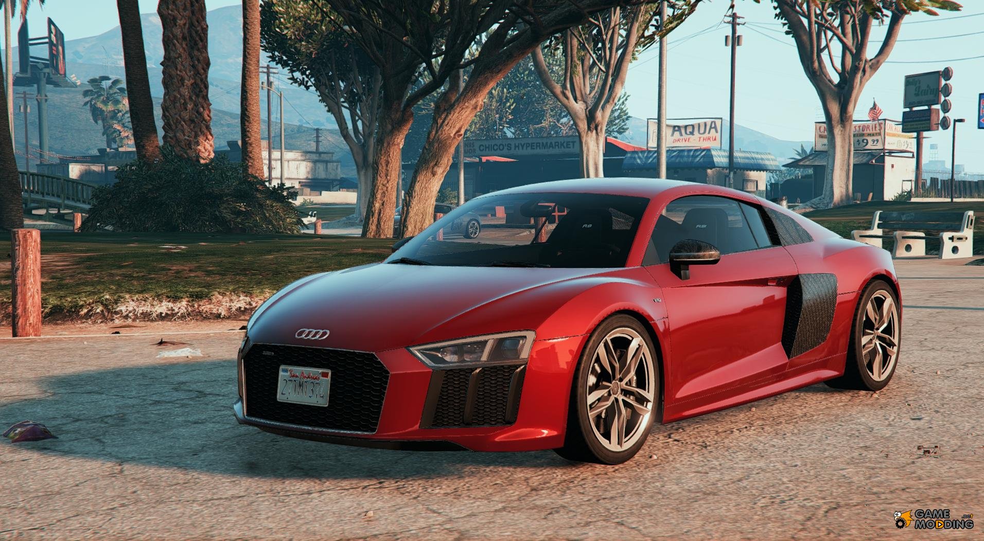
GTA5 is an early example of using this kind of single shader to render a range of materials.

Groundwork

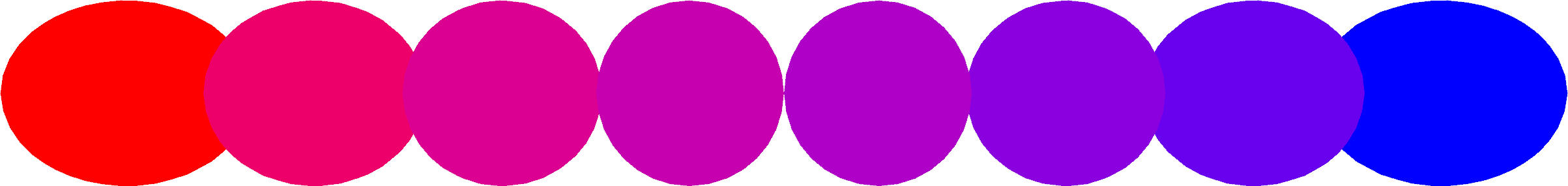
The ‘Lerp’ Function

Lerp is a very common function in graphics programming, it is built into all common shader languages. It takes two values and proportionally blends between them. We will make good use of this function

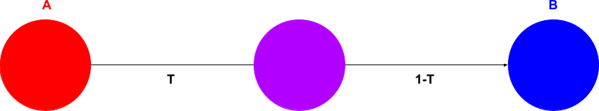
float3 lerp(float3 a, float3 b, float3 t)
{
    return a * (1-t) + b * t;
}

Bidirectional Reflectance Distribution Functions

When a process is bidirectional it is taking place in two, usually opposite directions. A BRDF is a function that gives the reflectance of a point on a surface given two directions, the direction of the viewer (Wr) and of the light (Wi).

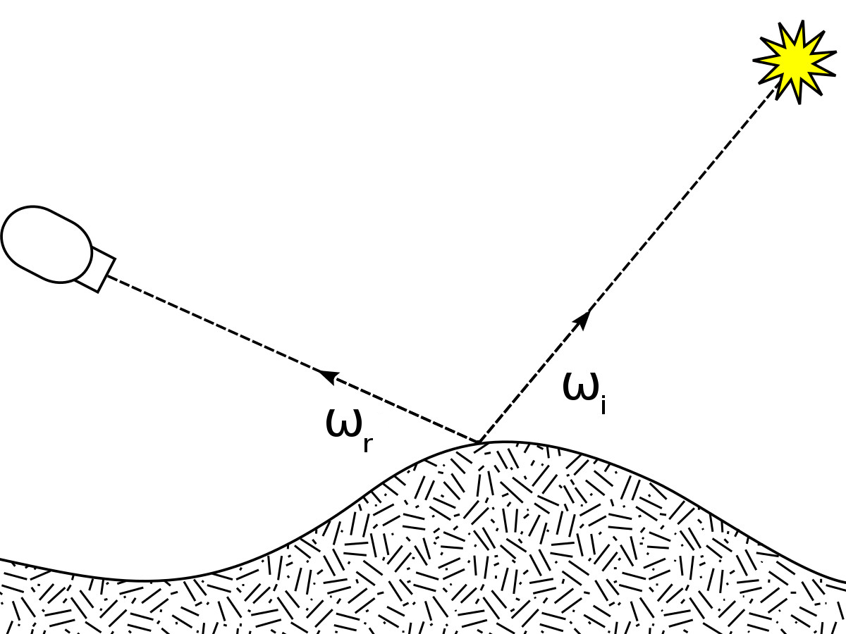
• source: ²

A BRDF returns the ratio of reflected light from the surface a viewer receives, this is known as the radiance. BRDF inputs Wr and Wi are usually defined as a pair of angles, azimuth (Φ) and zenith (θ), so the BRDF is considered a 4 dimensional function.

Measuring and recording the reflectance of a real surface is a difficult and time consuming process that uses a piece of equipment known as a gonioreflectometer. The MERL database records discretely sampled data in a BRDF lookup table for 100 different surfaces. Each MERL BRDF contains around 33mb of data.

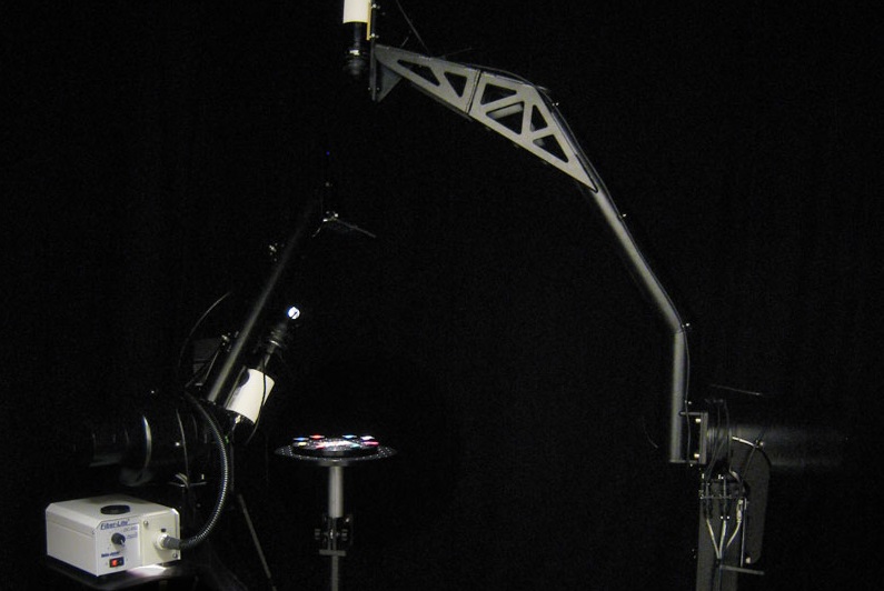
• source: ³

Instead of having to create large amounts of data for each surface we want to render, analytical models have been developed which, given some more parameters can approximate reflectance for a range of surfaces. Some well known ones are:

• Lambert
• Phong
• Cook-Torrance

For our purposes we will treat Wr and Wi as 3-dimensional vectors, to be passed as parameters to these functions.

Building Up a Model

Lambert is the simplest model here, while Cook-Torrance is considered physically based. Physically Based Rendering can include many different physical effects, but Cook-Torrance, or more accurately approximation of Cook-Torrance, contains the minimum necessary to be considered physically based and runs in real time. Cook-Torrance is equivalent to the PBR shading model found in Unreal engine and Unity 3D.

To see why this is we will build up from Lambert to Cook-Torrance approximation, step-by-step.

Lambert Shading

The lambert function models diffusion, which is when light slightly penetrates a material surface and is scattered uniformly. So we will call the result of the lambert function ‘diffuse’.

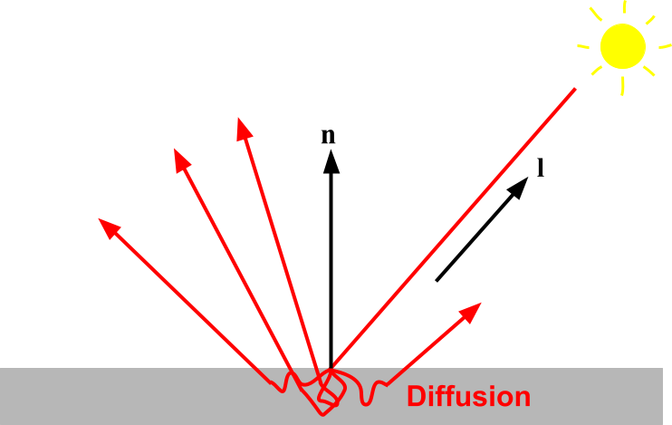
When considering a point light the Lambert function is just the dot product of the surface normal and light direction, clamped to above zero.

float3 diffuse_lambert(float3 n, float3 l)
{
    return max(0.0, dot(n, l));
}

Albedo colour

The ‘albedo’ term represents wavelengths of light absorbed by a material’s surface upon collision, what we typically understand as the surface colour.

float3 diffuse_lambert(float3 n, float3 l)
{
    return _Albedo.rgb * max(0.0, dot(n, l));
}

Shader

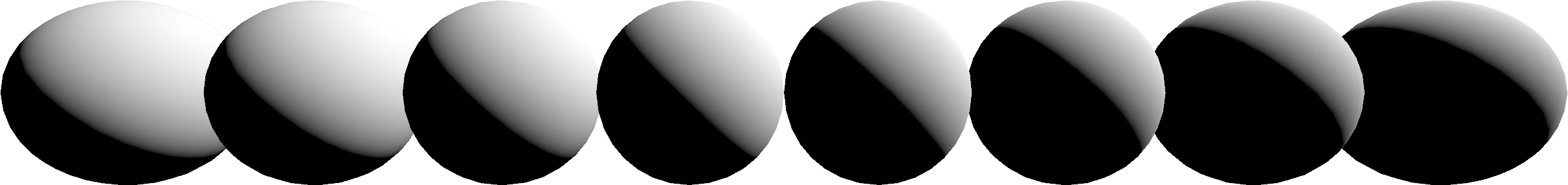
There are more accurate but more complicated diffuse models, but this one is simple and real-time fast, rendering an object just with this term is acceptable basic lighting. Still, we want to extend our model further.

float3 diffuse_lambert(float3 n, float3 l)
{
    return _Albedo.rgb * max(0.0, dot(n, l));
}

float4 frag (v2f i) : SV_Target
{
    float3 n = normalize(i.normal);
    float3 l = _WorldSpaceLightPos0.xyz - i.posWorld.xyz * _WorldSpaceLightPos0.w;
    //
    float3 diffuse = diffuse_lambert(n, l);
    //
    float3 output = diffuse;
    return float4(output, _Albedo.a);
}

Phong Shading

Light can also bounce directly off of the surface of a material, such as a mirror, without penetrating at all. Unlike diffuse light, this ‘specular’ light is dependent on the angle you are viewing from. For example look at a carpet and mover around a room and its lighting will not appear to move, but if you move around a mirror you will be able to see different parts of the room reflected as you move around.

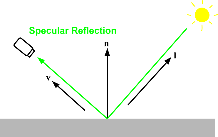
The new ‘v’ value is the viewing direction from surface to eye.

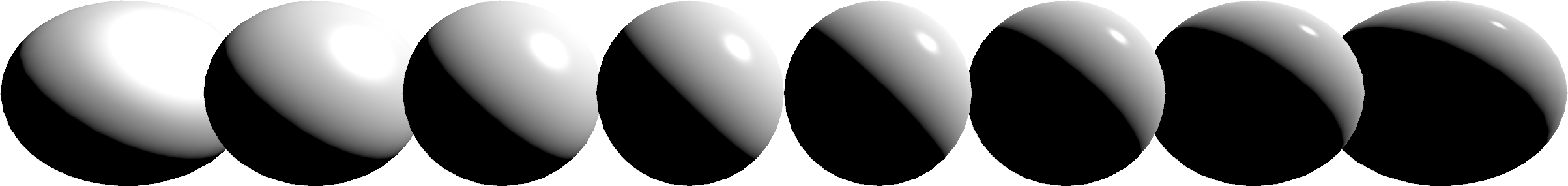
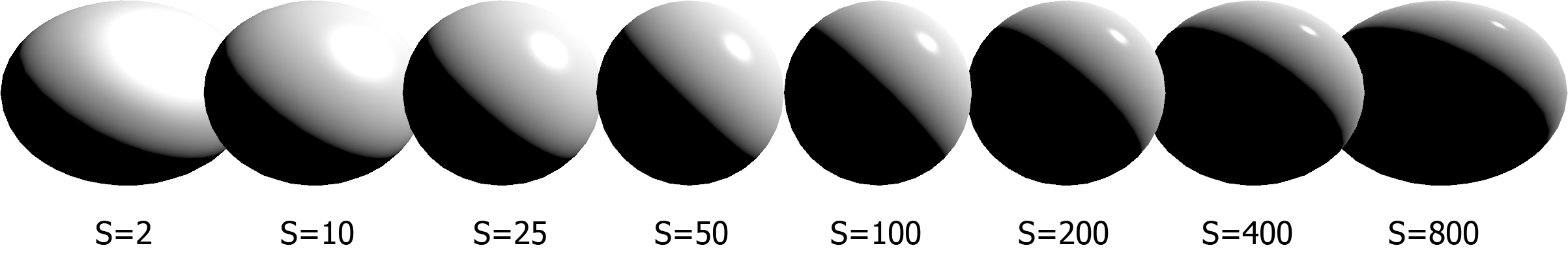
Shininess

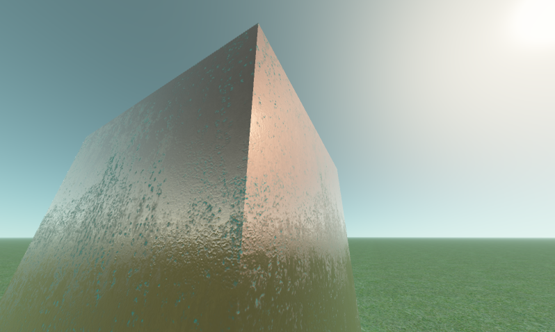
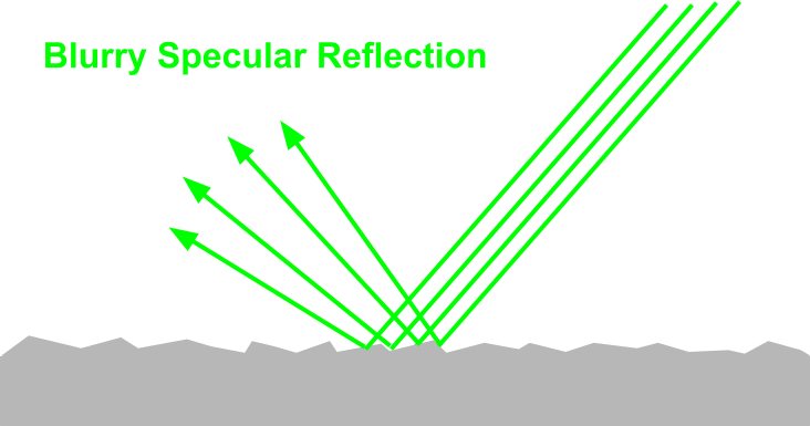
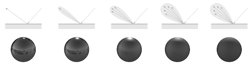
The Phong specular term takes a ‘shininess’ parameter which controls how much the reflection disperses light rays, and becomes blurry. Zooming in to see this surface much closer, unlike a smooth mirror reflection blurring is caused by microscopic roughness.

float3 specular_phong(float3 n, float3 l, float3 v)
{
    return pow(max(0.0, dot(reflect(-l, n), v)), _Shininess);
}

Unlike diffuse, in the Phong model specular reflection does not take any of the albedo colour, instead it takes the light colour. For the sake of simplicity the light colour has been left at white. This assumption does not hold for more complex models, as with Phong rendering a material which has a coloured reflection such as gold isn’t modeled.

Phong also does not model microscopic roughness well at all, this will be further explored building upon the Phong model.

Combining Terms

In Phong diffuse and specular terms are added together.

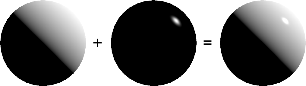
float3 output = diffuse + specular;

Shader

float3 diffuse_lambert(float3 n, float3 l)
{
    return _Albedo.rgb * max(0.0, dot(n, l));
}

float3 specular_phong(float3 n, float3 l, float3 v)
{
    return pow(max(0.0, dot(reflect(-l, n), v)), _Shininess);
}

float4 frag (v2f i) : SV_Target
{
    float3 n = normalize(i.normal);
    float3 l = _WorldSpaceLightPos0.xyz - i.posWorld.xyz * _WorldSpaceLightPos0.w;
    float3 v = normalize(_WorldSpaceCameraPos - i.posWorld.xyz);
    //
    float3 diffuse = diffuse_lambert(n, l);
    float specular = specular_phong(n, l, v);
    //
    float3 output = diffuse + specular;
    return float4(output, _Albedo.a);
}

Approximate Cook-Torrance

The Phong model contains two problematic heuristics.

• Diffuse and specular terms are added together, resulting in more light emitting from the surface than it receives.
• The shininess parameter is difficult to control, it varies non-linearly and ranges from zero to infinity.

Lets deal with both of these problems. It’s easier to think about these problems if we now switch to ‘image based’ rather than point lighting. Also, with the infinitely small point light it becomes invisible as the shininess parameter becomes perfectly mirror-like.

Two separate special lighting environment maps need to be generated from a regular environment map, this is done using offline tools such as Cmgen in Filament, which will bake the properties of the BRDFs in to new environment maps, this is what makes this model an approximation of Cook-Torrance rather than a direct implementation.

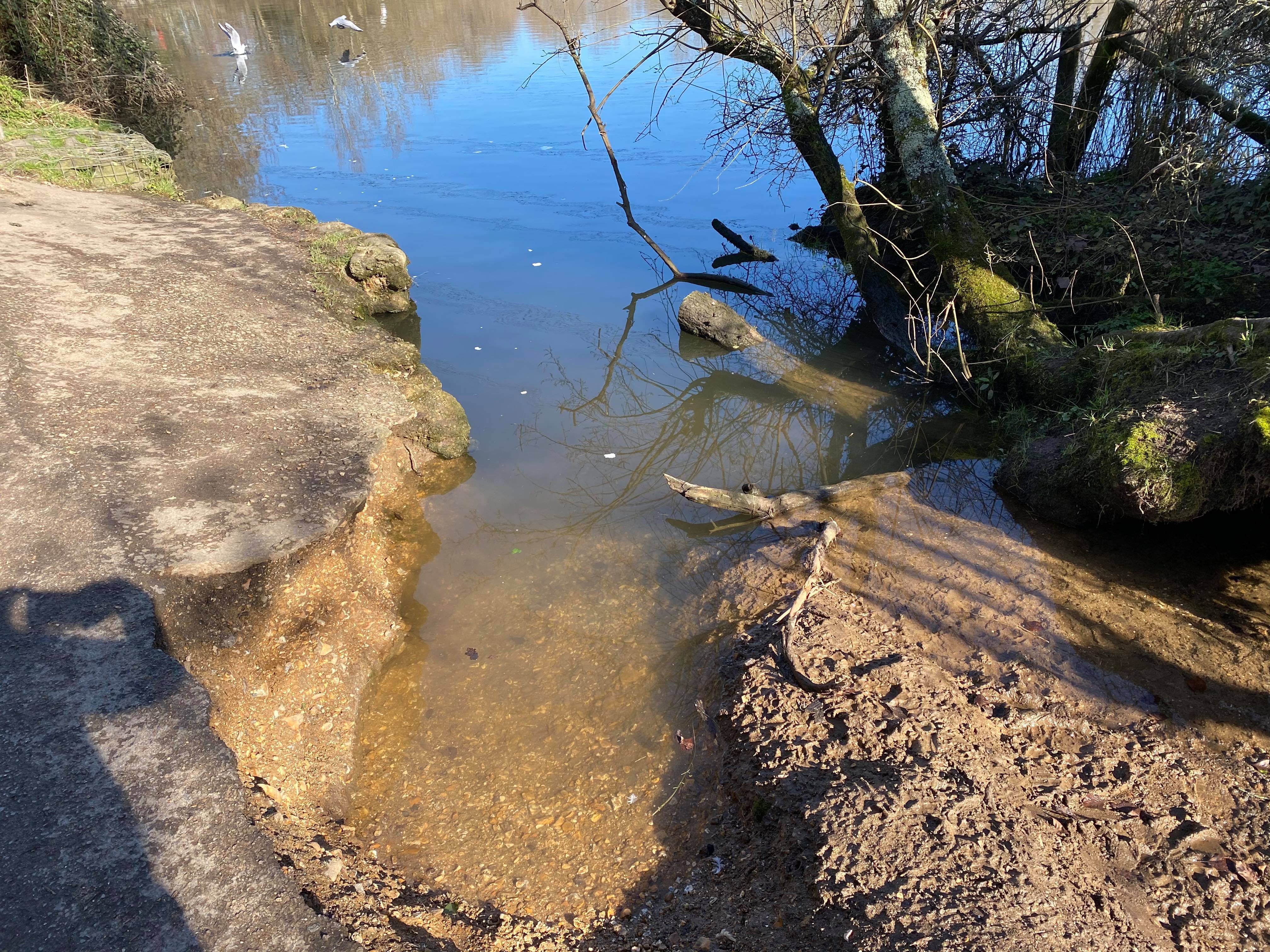
Here is our source ‘regular’ environment map.

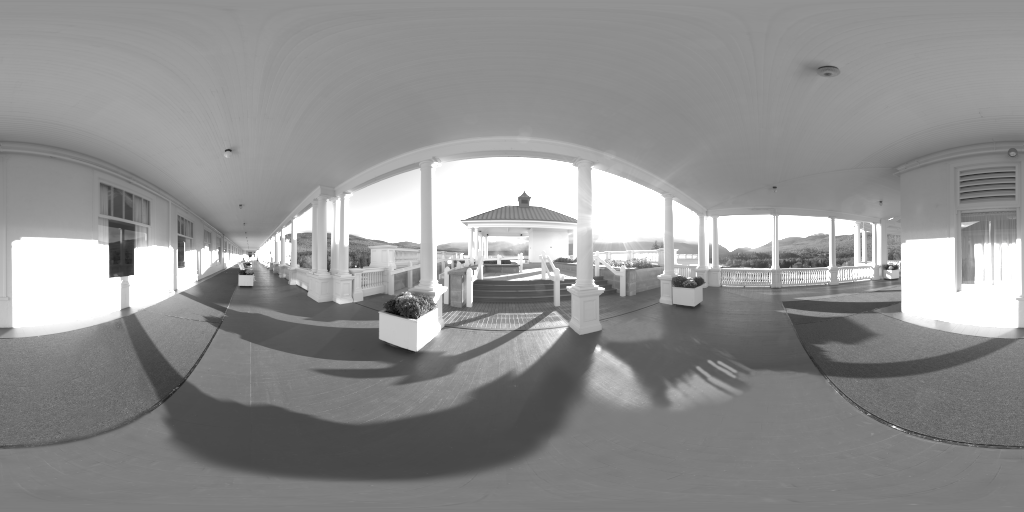
Image Based Diffuse Term

The ‘irradiance’ map is created by convolving the regular environment map.

Sampling the environment map for the image based diffuse term is straight-forward.

float3 diffuse_img(float3 n)
{
    return _Albedo.rgb * texCUBE(_IrradianceMap, n).rgb;
}

Image Based Specular Term

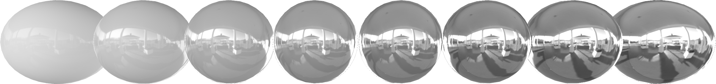
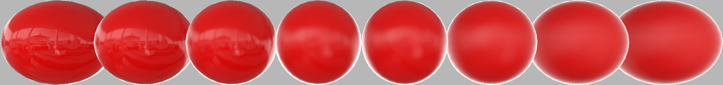
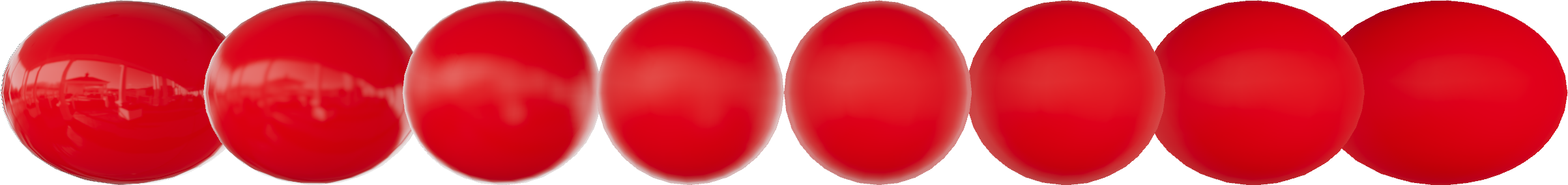
The ‘radiance’ map for specular reflections is baked into the mapmaps of an environment map, so with increasing roughness a blurrier reflection can be looked up.

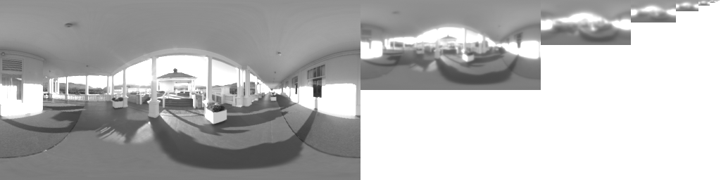
The shininess parameter is now named ‘roughness’, and varies nicely between zero and one. Much more understandable and controllable. Roughness now replaces the the difficult to control ‘shininess’ parameter.

float3 specular_img(float3 n, float3 v)
{
    float3 r = reflect(v, n);
    return texCUBElod(_RadianceMap, float4(r, _Roughness * MipLevelsInRadianceMap)).rgb;
}

Combining Terms

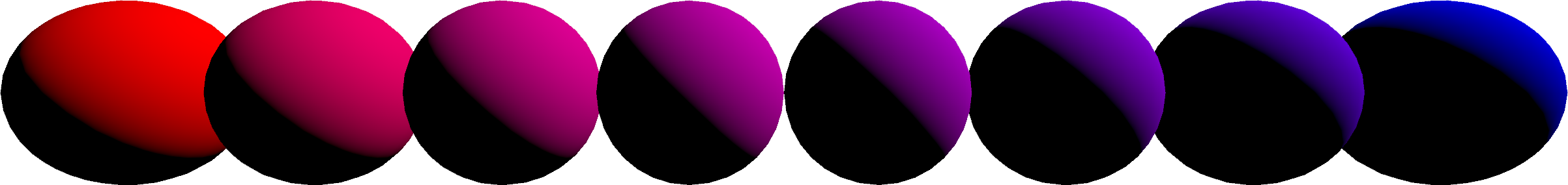
Instead of adding diffuse and specular terms, they should be blended with the Lerp function. This will give us a nice physically based property, conductivity to electricity. The parameter used to blend is called ‘metalness’.

float3 diffuse_img(float3 n)
{
    return _Albedo.rgb * texCUBE(_IrradianceMap, n).rgb;
}

float3 specular_img(float3 n, float3 v)
{
    float3 r = reflect(v, n);
    return texCUBElod(_RadianceMap, float4(r, _Roughness * MipLevelsInRadianceMap)).rgb;
}

float4 frag (v2f i) : SV_Target
{
    float3 n = normalize(i.normal);
    float3 v = normalize(_WorldSpaceCameraPos - i.posWorld.xyz);
    //
    float3 diffuse = diffuse_img(n);
    float specular = specular_img(n, v);
    //
    float3 output = lerp(diffuse, specular, _Metalness);
    return float4(output, _Albedo.a);
}

Combining Terms and Accounting for Albedo

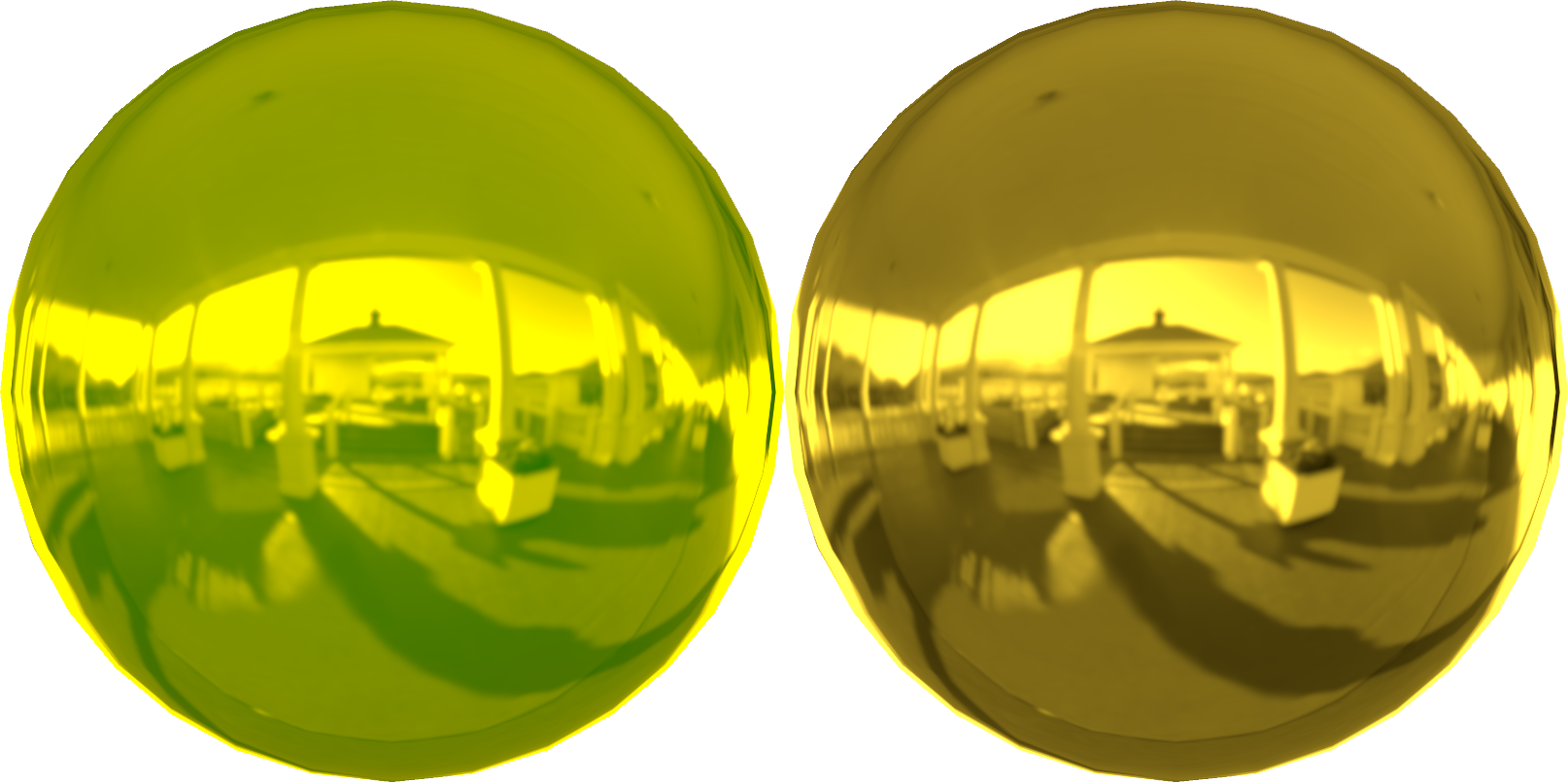
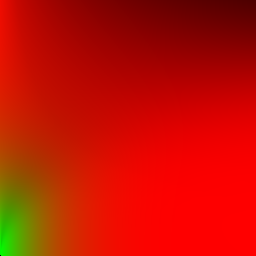
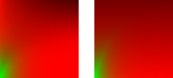
Coming back to the example of gold, a material that would not be convincingly rendered by Phong, we can now understand how to split up the albedo colour between diffuse and specular proportionally depending on conductivity. This is the ‘F0’ term which blends the specular and diffuse terms considering albedo colour and conductivity, which is clamped to a minimum of 4%, a value considered to be the lower bound for most real-world materials.

If the albedo colour was not split properly between specular and diffuse terms then energy conservation would be lost and a gold colour would appear an odd green hue.

float4 frag (v2f i) : SV_Target
{
    float3 n = normalize(i.normal);
    float3 v = normalize(_WorldSpaceCameraPos - i.posWorld.xyz);
    //
    float3 f0 = max(_Albedo.rgb * _Metalness, 0.04);
    //
    float3 diffuse = diffuse_img(n) * (1.0 - _Metalness);
    float specular = specular_img(n, v);
    //
    float3 output = lerp(diffuse, specular, f0);
    return float4(output, _Albedo.a);
}

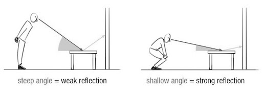
Fresnel and Energy Conservation

The Fresnel effect increases specularity and decreases the amount of albedo adsorption the more grazing the surface normal is to the viewer.

Incorrect Fresnel

The Schlick function can approximate an amount of Fresnel reflection very easily, however using it directly causes some issues.

float schlick(float f0, float f90, float NoV)
{
    return f0 + (f90 - f0) * pow(1.0 - NoV, 5.0);
}

float fresnel(float3 NoV)
{
    return schlick(0.0, 1.0, NoV);
}

float4 frag (v2f i) : SV_Target
{
    float3 n = normalize(i.normal);
    float3 v = normalize(_WorldSpaceCameraPos - i.posWorld.xyz);
    float NoV = dot(n, v);
    //
    float3 f0 = max(_Albedo.rgb * _Metalness, 0.04);
    //
    float3 diffuse = diffuse_img(n) * (1.0 - _Metalness);
    float specular = specular_img(n, v);
    //
    float3 output = lerp(diffuse, specular, f0 + fresnel(NoV));
    return float4(output, _Albedo.a);
}

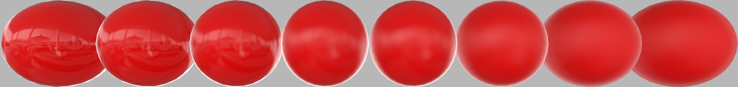
In this naive implementation, gold looks much better, it is now nicely achromatic around the edges and rendering of smooth materials looks much more convincing.

However, the problem now is rough surfaces glow brightly around the edges where they should not as roughness should be causing energy to dissipate, conservation of energy for grazing angles is lost.

Correct Fresnel

On a microscopic level small facets should mask and shadow light rays.

In this approximation of Cook-Torrance calculations are split and baked into the environment map, and in to a lookup table of Fresnel given surface roughness and viewing angle. This is the ‘split sum’ approximation.

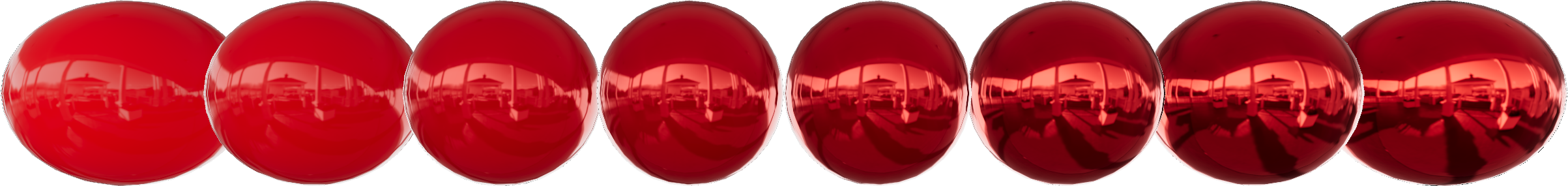
Using the lookup table for Fresnel term the bright halos are eliminated, restoring energy conservation for grazing angles.

Approximating the DFG Lookup Table

Instead of calculating this table and using up a texture sampler for it, this function below provides a reasonable linear approximation. It was developed for Unreal Engine 4.

// Approximates the roughness/Fresnel lookup table generated offline.
// Explained in Filament documentation.
// https://google.github.io/filament/Filament.md.html#table_texturedfg
float3 EnvBRDFApprox(float3 f0, float3 NoV, float roughness)
{
    float4 c0 = float4(-1.0, -0.0275, -0.572, 0.022);
    float4 c1 = float4(1.0, 0.0425, 1.04, -0.04);
    float4 r = roughness * c0 + c1;
    float a004 = min(r.x * r.x, exp2(-9.28 * NoV)) * r.x + r.y;
    float2 AB = float2(-1.04, 1.04) * a004 + r.zw;
    return f0 * AB.x + AB.y;
}

Fresnel with Lookup Table

float4 frag (v2f i) : SV_Target
{
    float3 n = normalize(i.normal);
    float3 v = normalize(_WorldSpaceCameraPos - i.posWorld.xyz);
    float NoV = dot(n, v);
    //
    float3 f0 = max(_Albedo.rgb * _Metalness, 0.04);
    //
    float3 diffuse = diffuse_img(n) * (1.0 - _Metalness);
    float specular = specular_img(n, v);
    //
    float3 output = lerp(diffuse, specular, EnvBRDFApprox(f0, NoV, _Roughness));
    return float4(output, _Albedo.a);
}

Rendering to a Display

Gamma

Computer monitors display RGB colour on a logarithmic scale, ‘gamma’, where a value of 50% does not represent half brightness. This is done because eyes are much more sensitive to dark colours so some more accuracy is assigned to the low range. The article The Importance of Being Linear from nVidia explains gamma space in-depth.

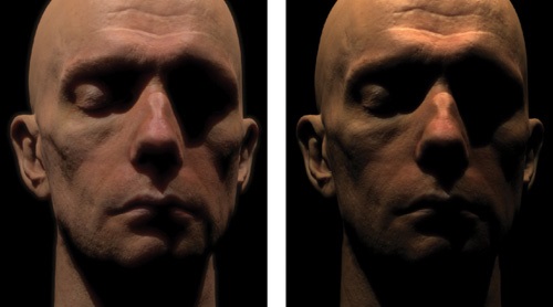
• source: ⁴

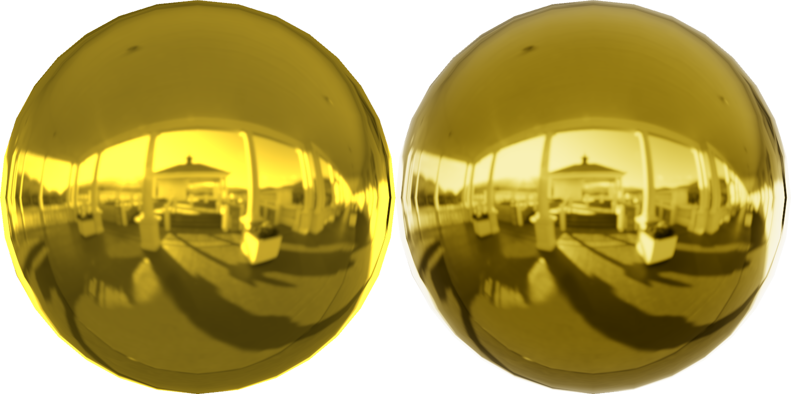
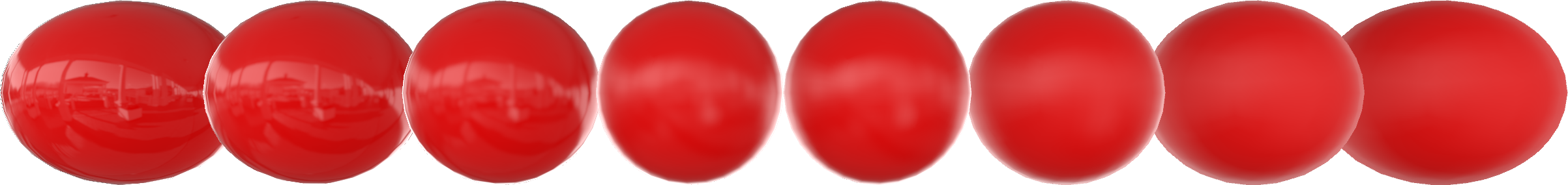
In the first image lighting is computed in the correct colour space, in the second linear values are not properly converted before display.

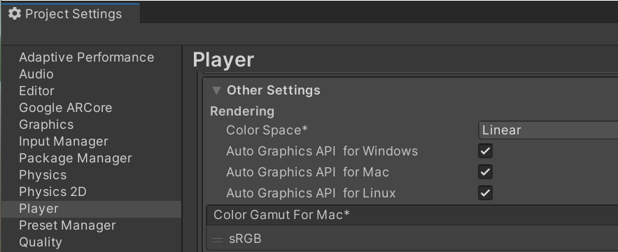
This shader is designed to output in linear colour space. To be correct Unity must be configured to match the shader output values, so automatic conversion to gamma space is done before display.

Tone Mapping

The output of our shader has a very high-dynamic range and needs to be mapped to a more suitable range for display on a screen. This is one such function, which unlike simpler ones is chroma preserving. Tone mapping functions are designed to mimic how film adsorbs light, a more in depth explanation can be found here.

//https://github.com/TheRealMJP/BakingLab/blob/master/BakingLab/ACES.hlsl

static const float3x3 ACESInputMat =
{
    {0.59719, 0.35458, 0.04823},
    {0.07600, 0.90834, 0.01566},
    {0.02840, 0.13383, 0.83777}
};

static const float3x3 ACESOutputMat =
{
    { 1.60475, -0.53108, -0.07367},
    {-0.10208,  1.10813, -0.00605},
    {-0.00327, -0.07276,  1.07602}
};

float3 RRTAndODTFit(float3 v)
{
    float3 a = v * (v + 0.0245786f) - 0.000090537f;
    float3 b = v * (0.983729f * v + 0.4329510f) + 0.238081f;
    return a / b;
}

// Maps real valued output to a suitable range for display on an
// 8-bits per channel RGB screen.
float3 toneMapACES(float3 color)
{
    color = mul(ACESInputMat, color);
    color = RRTAndODTFit(color);
    color = mul(ACESOutputMat, color);
    color = saturate(color);
    return color;
}

return float4(ToneMapACES(output), _Albedo.a);

Exposure Control

Along with the tone mapping it can be useful to mimic ‘shutter speed’, to control how exposed the film is.

return float4(ToneMapACES(output * _Exposure), _Albedo.a);

GitHub Gist

float4 frag (v2f i) : SV_Target
{
    float3 n = normalize(i.normal);
    float3 v = normalize(_WorldSpaceCameraPos - i.posWorld.xyz);
    float NoV = dot(n, v);
    //
    float3 f0 = max(_Albedo.rgb * _Metalness, 0.04);
    //
    float3 diffuse = diffuse_img(n) * (1.0 - _Metalness);
    float3 specular = specular_img(n, v);
    //
    float3 output = lerp(diffuse, specular, EnvBRDFApprox(f0, NoV, _Roughness));
    return float4(ToneMapACES(output * _Exposure), _Albedo.a);
}

Appendix

Radiometric Units

As integrating over a hemisphere means somehow summing up over all possible angles, and dividing by pi. So a division by pi should really be factored in to light colour to be fully energy conserving.

float3 diffuse_img(float3 n)
{
    return _Albedo.rgb * (1.0 \ 3.142) * texCUBE(_IrradianceMap, n).rgb;
}

float3 specular_img(float3 n, float3 v)
{
    float3 r = reflect(v, n);
    return texCUBElod(_RadianceMap, float4(r, _Roughness * MipLevels)).rgb * (1.0 \ 3.142);
}

Introducing the pi division means lighting units are supplied in terms of luminous flux (lumens) instead, which is harder for an artist to work with. Particularly for games the division is simpily dropped to make lighting input units normalized to 1.

Environment Map Representations

Real Time Rendered Environment Cubemaps

It might not always be possible to use a baked environment map, sometimes a more dynamic scene is needed and environment maps need to be updated at runtime. A dynamic environment cubemap can be used to approximate a pre-baked one with some lookup adjustments.

Irradiance Map

The 2nd to last mipmap level of an environment cubemap rendered at runtime can make a suitable approximation of the pre-rendered map.

Radiance Map

Further work is needed to calculate which mipmap level to look up. The size mipmaps grow each level must be accounted for with ‘log2’, whereas with the pre-baked map this is already accounted for.

ComputeReflectionCaptureMipFromRoughness in Unreal Engine 4

half ComputeReflectionCaptureMipFromRoughness(half Roughness, half CubemapMaxMip)
{
    half LevelFrom1x1 = REFLECTION_CAPTURE_ROUGHEST_MIP - REFLECTION_CAPTURE_ROUGHNESS_MIP_SCALE * log2(Roughness);
    return CubemapMaxMip - 1 - LevelFrom1x1;
}

Point Lights

Phong shininess can be fitted to be linear, mapping to micro surface rougness. Epic publishes their fitting for Unreal Engine 4. D_Approx replaces EnvBRDFApprox.

half D_Approx(half Roughness, half RoL)
{
    half a = Roughness * Roughness;
    half a2 = a * a;
    float rcp_a2 = rcp(a2);
    // 0.5 / ln(2), 0.275 / ln(2)
    half c = 0.72134752 * rcp_a2 + 0.39674113;
    return rcp_a2 * exp2( c * RoL - c );
}

Irradiance as Spherical Harmonic

Sometimes irradiance can be stored as a spherical harmonic, of 9 terms with 3 colour channels. Passing in a direction normal will return the irradiance in that direction.

static float3 SH[] =
{
    float3(0.532722413539886, 0.532722413539886, 0.532722413539886),
    float3(0.055692940950394, 0.055692940950394, 0.055692940950394),
    float3(-0.064554333686829, -0.064554333686829, -0.064554333686829),
    float3(-0.012459455989301, -0.012459455989301, -0.012459455989301),
    float3(-0.022898603230715, -0.022898603230715, -0.022898603230715),
    float3(0.128989517688751, 0.128989517688751, 0.128989517688751),
    float3(0.066114954650402, 0.066114954650402, 0.066114954650402),
    float3(-0.054822459816933, -0.054822459816933, -0.054822459816933),
    float3(0.065103121101856, 0.065103121101856, 0.065103121101856)
};

float3 diffuse_sh(float3 n)
{
    return max(
        SH[0]
        + SH[1] * (n.y)
        + SH[2] * (n.z)
        + SH[3] * (n.x)
        + SH[4] * (n.y * n.x)
        + SH[5] * (n.y * n.z)
        + SH[6] * (3.0 * n.z * n.z - 1.0)
        + SH[7] * (n.z * n.x)
        + SH[8] * (n.x * n.x - n.y * n.y)
        , 0.0);
}

References